Data and Methods
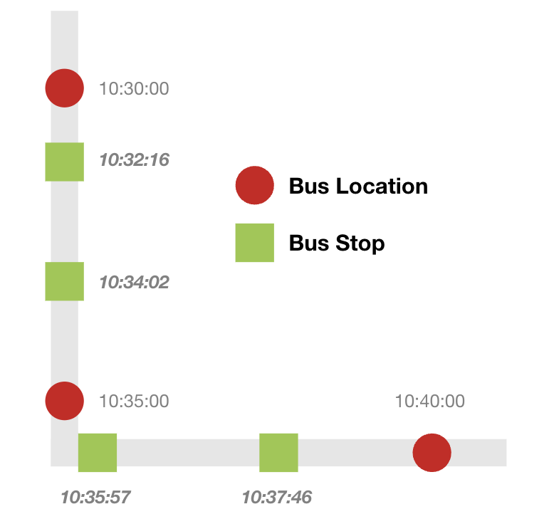
The Mansueto StopWatch is centered around the bus stop. We picked this unit of analysis since it constitutes the main point of contact between users and bus service: the stop is where users wait for the bus and it determines how close the service is from their trip origin and destination. Since there is no public data that precisely shows when a bus stopped at a bus stop, our first and major technical challenge was to build such data set. This would then be the building block for the aggregated metrics. To produce the data set, we took a variety of steps to process and merge several data sources, such as community, bus stop and route shapefiles, historic bus location pings, and the historic bus schedule data.
For the breakdown of how we process these inputs, we follow the terminology used by the CTA API documentation:
- Route: A collection of patterns
- Pattern: One possible set of stops that a bus can travel on
- Trip: For a given pattern, a buses journey from the first stop to the last stop
We began with over 110 million real time bus locations from June 1st 2022
to July 28th 2024 as provided by the
Chi Hack Night Ghost Bus
project. These bus locations are real-time data from the
CTA bus tracker API
get vehicles feed, which stores real-time data
queried every five minutes. Each bus location ping includes
metadata such as vehicle number, route, pattern id, and a trip
id. Due to the lack of uniqueness of the existing trip ID provided, we
created a unique trip ID to group a collection of bus locations together.
Each trip represents a specific bus on a specific pattern and route at a
certain time of the day (for example, bus with vehicle ID 4654 traveling
northbound on pattern 1456 on route 6 on June 30th, 2023.) While this
method is not perfect, this new trip ID allows us to group bus pings
into one trip which facilitates analysis of service reliability.
Using this method, we identified 10,235,984 unique trips in the original
data set. For our analysis, it was necessary to transform the raw bus
location data into the desired bus stop view.
The original data represents 5-minute snapshots of
every bus in the CTA system which was converted to the times that each bus
passes a bus stop using imputation. For example, if two buses pass a stop within a 5-minute
snapshot, there will be two rows, each listing the estimated time the
first bus passed a stop and the estimated time since the last bus. This
transformation is necessary as it allows us to derive performance metrics
that are more interpretable and easier to localize than bus positions.
To do this, we
- Determined the bus stops for a particular trip by using the pattern ID and bus stop locations as provided by the CTA
- Combined bus locations and stop locations for a trip spatially
- Removed bus locations that were not on route
- Interpolated the time a bus arrived at a bus stop by using the time and distance between bus locations and the distance from bus stops between the bus locations
We then processed historic schedules of bus service to contrast it with the actual service provided. For this purpose, we used General Transit Feed Specification (GTFS) data. The CTA only allows for the download of the current schedule, which was an obstacle considering that we planned to evaluate bus service going back to June 2022. However, Transit land, an open data platform that collects GTFS data, maintains historic archive of all feeds. Historic feeds back to May 2022 were downloaded. Schedules were recreated from this historic GTFS data using GTFS Kit, an open-source Python library to work with GTFS data.
In addition to bus pings and schedules, the analysis relies on shapefiles of three main units of analysis: community areas, bus stops and routes. These shapefiles are mainly used for visualizations and for spatial operations. More specifically, we performed point-in-polygon operations to aggregate service performance metrics at the community level—by identifying the bus stops that serve each of the 77 community areas. Up-to-date shapefiles are available at the Chicago Data Portal for the following spatial units:
Using both the historic real-time bus location and the historic schedule data bus stop level, we calculated the following metrics for different time periods (including hour of the day, day of the week, week of the year, month of the year, year, week for each given year and month for each given year).
Metrics include:
-
Time to next bus stop
- Given a bus is at a bus stop, the time until the next bus on the same route arrives.
-
Excess Time to Next Bus
- The actual time to next bus minus the scheduled time to next bus
-
Trip Duration
- The time difference between the first and last stop.
-
Trip Delay
- The actual trip duration minus the scheduled trip duration.
-
Number of buses
- How many buses passed a bus stop in each time interval
-
Excess number of buses
- Actual number of buses in each time interval minus scheduled number of buses
To calculate the metrics, we:
- Filter to only trips with stops between 6am and 8pm
- Calculate the median, mean, standard dedication, max, min, 25 quartile, and 75 quartiles for each metric.
- Aggregate to the route and community area level to varying time periods by findings the weighted median value of the metric for each stop using the number of buses that pass each bus stop in the aggregation unit.
For further details on the project data and methodology, consult the full report or the code repo.
Access these comprehensive metrics, updated daily covering all stops here.
